APTOS 2019 Blindness Detection
Overview
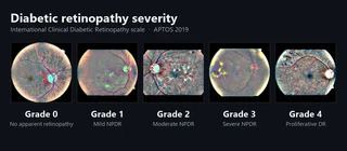
The APTOS 2019 Blindness Detection Kaggle challenge asks contestants to grade diabetic retinopathy (DR) severity from a single retinal fundus image according to scale represented by five ordinal classes, following the International Clinical Diabetic Retinopathy (ICDR) severity scale:
| Grade | ICDR label | What a grader is looking for |
|---|---|---|
| 0 | No apparent retinopathy | no evidence of abnormalities |
| 1 | Mild NPDR | microaneurysms only |
| 2 | Moderate NPDR | more than microaneurysms, less than severe |
| 3 | Severe NPDR | the “4-2-1” rule — haemorrhages in 4 quadrants, venous beading in 2+, or IRMA in 1+ |
| 4 | Proliferative DR | neovascularisation, vitreous or preretinal haemorrhage |
Further information on this scoring can be found on PubMed here
Predictions for this competition were scored by quadratic weighted kappa (QWK), a statistical metric that measures the agreement between two raters classifying something represented by an ordinal scale. Ordinal as in items that have some logical ordering. A score of 1 represents perfect agreement and a score of 0 is bad.
External data was allowed, so the 2015 Diabetic Retinopathy dataset could be used. My competition entry reached a public leaderboard score of 0.816, not that it mattered as I forgot to then select a score for the final private leaderboard scoring!! All is good though, I welcomed my newborn baby into the world and became a dad instead!
The most interesting part of the project was what it taught me about medical imaging and the differences between a better image and a better label.
My Walkthrough
I started from a notebook recipe that was circulating on Kaggle at the time and then explored a few parts that I had opinions about.
- Preprocessing The Ben-Graham crop — A protocol that finds the circular fundus, crops to it, then subtracts a local average of the colour to flatten uneven illumination — plus a resize to 224px. This is the smallest resolution that pre-trained EfficientNet’s could support, I only had a 1080ti at the time locally to work with and wanted faster turnaround times for experiments
- De-Duplication It was suspected collectively from contestants that some images from the 2015 dataset were part of the 2019 dataset, mainly due to large local CV scores compared to the public test leaderboards. Typical practice is to use a perceptual-hash audit across datasets, and then remove duplicates.
- Backbone EfficientNet-B0 with CBAM (Convolutional Block Attention Module) grafted in. The goal was to exploit transfer learning from B0’s imagenet weights, fine-tune on the 2015, then further fine-tune again on the 2019 dataset.
- Cross-validation A 5-fold
StratifiedKFoldprotocol to measure baselines against the public test leaderboard scores. - Loss heads I explored all the losses. Cross-entropy, focal, Lovász and ordinal heads, plus an MSE regression head on the label treated as a continuous value. No loss really dominated
- Certainty-aware inference For each fold I ran 50 repeated forward passes with dropout enabled and kept, per image, the mean class probabilities and the standard deviation across passes. This was a cheap uncertainty estimate that I used for both model selection prior to stacking, and later for gating the pseudo-labels to QWK scores.
- Stacking I had wanted to try stacking from the beginning of this competition, this had been proven effective from other competitive solutions in the past. So I trained XGBoost over the five class probabilities, then used a Rounder further optimized to fit ordinal thresholds for maximizing QWK rather than assuming equidistant scoring intervals 0.5/1.5/2.5/3.5.
I did accumulate a few dead-ends on the research side, mainly across different architectures (UNets, Inception-CBAM, AttentionResnet, InceptionResnet, etc.). I did look to see if augmentations could be optimized i.e. what improved and what didn’t to the scores, but this was just too uncertain. The one experiment worth writing about is the one that failed for a conceptual reason rather than a technical one which I’ll elaborate on next.
The “Haze” Removal Experiment
The reasoning that got me started on this experiment was straightforward. Looking at all the Fundus photographs, I could see they had a fogginess haze to them. Low contrast, with a light grey-whitish wash. I found there is a well-established algorithm to solve that problem in digital photographs. Dark Channel Prior (DCP) by He, Sun & Tang. This algorithm notably won CPVR’s best paper award in 2009. My hypothesis was that if a dehazing step sharpened the retinal detail, the classifier would do better.
I connected up four separate DCP implementations a naive per-pixel one, a Numba one, a pure-NumPy one, and finally the one I actually used, which leaned on OpenCV’s capabilities for speed.
The protocol was to first crop the black border, detect the optic disc with a Hough circle algorithm so that every image was centred and scaled consistently, then run DCP over the images. I ran it over both the 2015 and 2019 training data successfully, then trained with the rest of the pipeline on the dehazed sets.
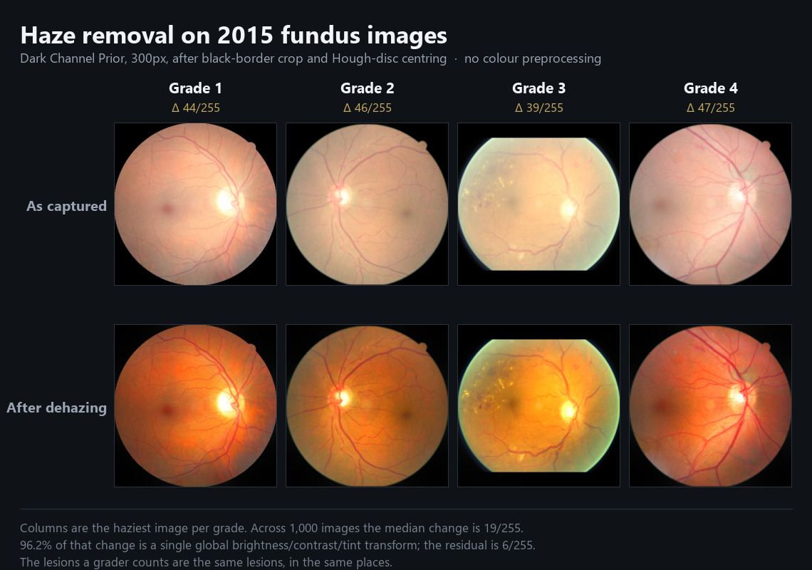
The same pipeline on the 2015 set. Columns are the haziest image per grade. The change here is roughly three times larger than on 2019, and the bottom row shows why the tone row of the table matters: it is mostly saturation and contrast.
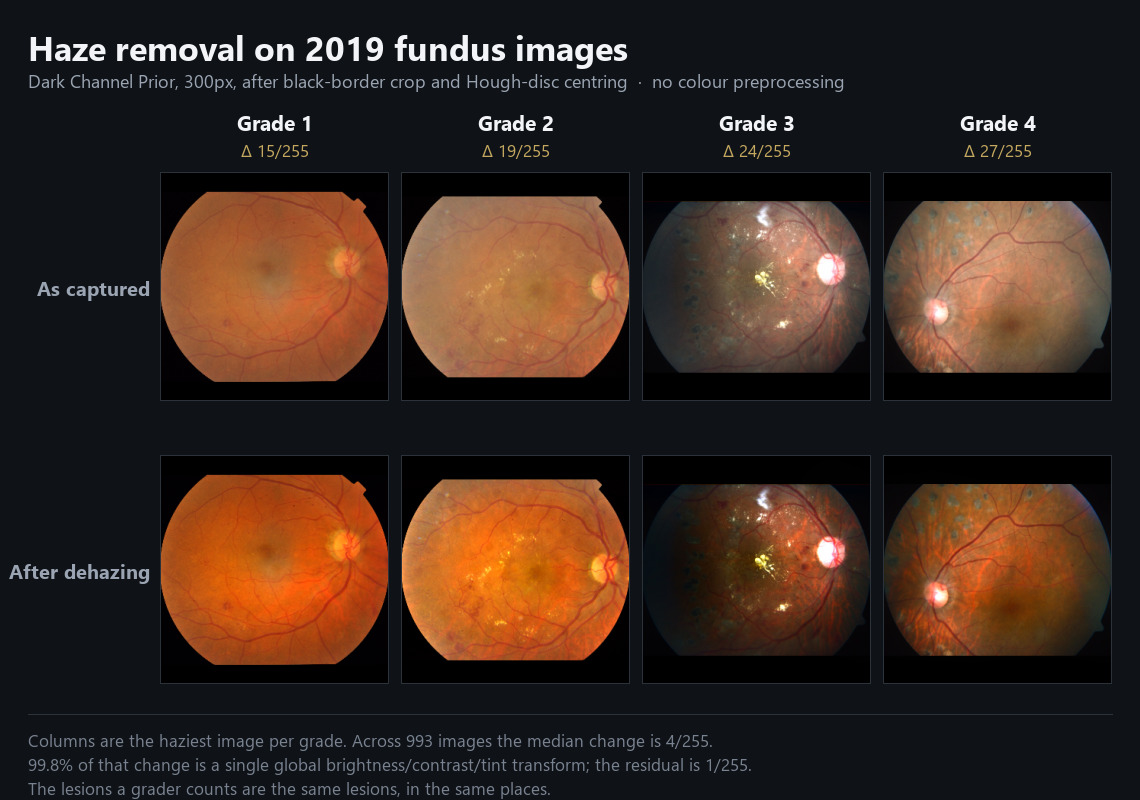
Before and after Dark Channel Prior on the four haziest images in the 2019 set — the dehazer at its strongest. Top row as captured, bottom row dehazed. Each column is labelled with the mean absolute pixel difference.
Ok great, much more vibrant images!
But, when I evaluated the impact of that change, I scored worse on validation sets with dehazed images, than compared to the original as captured ones.
Why it was never going to work
Pondering why the dehazing experiment failed so badly, it occurred to me that obviously the labels are a humans diagnosis of the fundus image as it was shown to them. Clinicians and trained graders look at thousands of these images, haze and all and assign a severity score regardless. It is possibly that a grader may struggle to see markers that lead to a particular severity conclusion, but the QWK metric scores the agreement between grades, not the quality or accuracy of the grade itself. The scale remains a qualitative assessment anyway.
Diabetic retinopathy is not graded by how sharp or clean a photograph is. Its performed by identifying and counting specific lesions. So the assumption I had was wrong. I assumed a direct correlation between image quality and label quality.
What I Learned
The technical lesson I walked away with was more about the challenges associated with AI based medical labelling in general. When the target is based upon a clinician’s judgement, the ceiling is set by the judgement, not by the quality of imaging or medical report that led to that judgement. Sure it might help the human judgement be more accurate for a patients sake, catching disease early enough such that treatment becomes more effective. But for AI systems to be designed well enough for widespread medical usage, they have to be robust for all kinds of flaws and diversity seen across the data itself. This framing has stayed with me all these past years since.
Techniques Used for my Final Submission Pipeline
- Preprocessing — Ben-Graham crop and local-average colour subtraction, 224px, with duplicate auditing across the 2015 and 2019 sets
- Two-stage training — pretrain on the 2015 dataset, then fine-tune on APTOS 2019 with 5-fold
StratifiedKFold - Model selection — a
val_QWK − val_losscallback rather than validation loss alone, since QWK is the competition metric - Certainty-aware inference — 50 repeated forward passes per fold to get stable mean class probabilities plus a per-image standard deviation
- Test Time Augmentation - Instead of performing 50 repeated passes on the full test dataset, fundus images were rotated 45-degrees 8 times instead. This was naturally a lot faster obviously.
- Ensembling — mode-vote across the five folds
- Stacking — XGBoost regressor over the class probabilities, then an OptimizedRounder fitting ordinal thresholds directly to QWK
- Certainty-gated pseudo-labeling — keep test images where the ensemble and the stack agree and certainty is high (ran, but the retrain never completed)
